Tuning Image Classifiers using Human-In-The-Loop
We present an Expectation–Maximization (EM) algorithm for iteratively estimating the optimal class-confidence threshold for an image classifier using human annotators. The algorithm is developed for classifiers that are applied to out-of-distribution images, and efficiently constructs a validation data set to estimate an optimal threshold for this use case.

Senior Applied Scientist
In this blog post we describe an algorithm we developed when building our product image analysis infrastructure, where we use human-in-the-loop to tune the thresholds of our image classifiers. We discuss the algorithm in the following, and present some mathematical details and a simple code example in the appendices.
Background
When a customer browses for a product on the Zalando website they may use descriptive terms to search for what they want, for example a customer may use a specific term such as leopard print dress instead of providing a more generic term such as casual dress. One approach we use to support product search using descriptive terms is to automatically generate additional product information from product images using computer vision techniques. In particular, we train image classifiers to identify products that have a particular fashion attribute such as a specific pattern or style, e.g. leopard print, which correspond to descriptive search terms.
Problem
A typical image classifier generates a class-confidence score (a value between 0 & 1) at its output to indicate that a given input image belongs to one of the specified output classes, i.e., the image shows a particular fashion attribute. To generate a binary decision from the classifier output a class-confidence threshold parameter is selected based on a classifier performance metric such as precision & recall. Once the threshold has been selected the model can be deployed and used to generate class labels for an input image, which can be used in product search.
Over time the characteristics of the input product images may change, leading to a drift in the input data distribution. For image classifiers that are used to generate predictions for out-of-distribution input images the performance of the classifier may degrade. For example this may occur when an image classifier is trained on Zalando product images before the introduction of a new photography style on a revamped Zalando website, for which there are no annotated image examples in the new style available to retrain the model.
To solve this problem we modify the class-confidence threshold of the classifier to compensate for data distribution drift, and developed an Expectation-Maximization (EM) algorithm that we call AutoThreshold for this purpose. AutoThreshold estimates an optimal class-confidence threshold for an image classifier using manual annotations from a selection of the classifier's predictions on the out-of-distribution data. Additionally, the process of creating annotations for the out-of-distribution data helps in the generation of a new data set that can be used to train a new version of the image classifier.
Selecting Classifier Thresholds
The optimal threshold value for an image classifier is the class-confidence score, a value between 0 & 1, for which the set of predictions above that score leads to optimal classifier performance. Ideally this value would be 0.5, i.e., the center of the range. However, for a number of reasons this is never the case and is usually estimated post training to achieve best results.
The estimated optimal threshold for each output class of an image classifier is evaluated using an annotated image data set, i.e. validation set, where each image in the set is manually assigned a class label. The image classifier is tested by using the validation data set as input and comparing the classifier's predictions to the manually assigned labels. We can measure classifier performance using metrics such as precision & recall, which indicate the quality and quantity of the results. Optimizing the threshold is usually a tradeoff between precision & recall, where we want to find a threshold value that results in an acceptable score for both. Typically, a performance metric that combines both precision and recall, such as the \(f_\beta\)-measure, is used, and the class-confidence score that maximizes the metric is chosen as the threshold value.
Estimating Thresholds in the Absence of Data
For our use case there exists no training or validation data set for the out-of-distribution input image set. Furthermore, we do not annotate all images in advance, as this would be a costly, and time consuming, exercise for the scale of the data at Zalando (currently around 600k products). To overcome these issues we make use of the simple fact that when classifier predictions are ordered by class-confidence score—for a well trained image classifier—high-confidence class predictions exhibit greater correspondence with the image annotations than low-confidence predictions, which indicates model performance, and allows us to search for an optimal threshold between both extremes (demonstrated in the plot below). With this in mind, we frame threshold selection as an optimization problem using manual annotators, who generate annotations to be used in the metric calculations required to estimate a threshold.
Specifically, we take an iterative approach, where images to be annotated are conditioned on the image classifier, and annotators annotate a subset of the classifier's most confident predictions first. The generated annotations are used to estimate a threshold using our selected performance metric, and the process is repeated until our estimated threshold converges. This process can be implemented as an Expectaton-Maximization algorithm, and describes a human-in-the-loop procedure, which generates a validation data set for the out-of-distribution data over a number of iterations. Furthermore, the data set is generated in an efficient way, both in terms of the number of annotations required, and the selection of image examples which contribute most to discovery of an optimal threshold.
Problem Definition
Taking a binary image classifier as our motivating example, which typically has a sigmoid output layer, the value generated at the output for each of the \(n\) input images can be interpreted as a class-confidence score, or probability \(p_{i}\), that an input image, \(\mathbf{x}_i\), belongs to the output class, \(c\). For the purposes of image attribute identification, the predictions at the output, \(\mathbf{p} =[p_{1},\dots,p_{n}]\), undergo a thresholding operation to replace the class-confidence scores with a binary class label, which indicates a transform from a continuous to categorical probability distribution. Since the output layer is a sigmoid function, where output values are thresholded by the parameter \(t\) into two binary categories, true & false, we can model the classifier's output distribution using a Bernoulli distribution, i.e., \(P(\mathbf{x}_i=c | p_{i})\). Furthermore, the distribution of annotations also follows a Bernoulli distribution. Using these details, we frame the problem of threshold estimation within the framework of the Expectation-Maximization algorithm, where we present algorithm details below, and present a more detailed mathematical explanation in Appendix A.
Threshold Estimation Using the EM Algorithm
The Expectation-Maximization algorithm is an iterative method to find maximum likelihood estimates of parameters (such as our classifier threshold) in the presence of unobserved latent variables. In our problem setting, the predictions made by the classifier are observed by our annotators to generate image annotations. However, the order of the images presented to the annotators is conditioned on the classifier's class-confidence score, which is unknown to our annotators. As mentioned, the estimated optimal threshold corresponds to a class-confidence score, and thus our latent variable allows us to estimate an optimal threshold for our classifier. Each iteration of the EM algorithm alternates between performing an Expectation step (E-step), which constructs a likelihood function to estimate the latent variable, and a Maximization step (M-step), which computes parameters that maximize the function constructed in the E-step. For our algorithm, the E-step generates annotations for the classifier's most confident predictions and the M-step estimates the optimal class-confidence threshold using the new set of annotations. Both steps are repeated at each iteration until the estimated threshold converges.
Algorithm Details - Binary Classifier
For a set of images, \(\mathbf{X}=[\mathbf{x}_1,\dots,\mathbf{x}_n]\), and their class-confidence scores, \(\mathbf{p}\), we construct a set of images ordered by their scores, \(\mathbf{X}_{\tt asc} = {\tt sort}(\mathbf{X},\mathbf{p})\), to estimate the optimal threshold, \(\hat{t}\), for the output class. We use \(\mathbf{X}_{\tt asc}\) as input to the AutoThreshold algorithm, and specify a number of hyperparamters including the subset window size \(m\), and classifier performance metric \({\tt metric}(.)\) (e.g., \(f_{\beta}\)-measure). We define a data windowing function that selects images to be annotated by centering a window of size \(m\) on \(\mathbf{X}_{\tt asc}\) at a position that corresponds to current threshold estimate (class-confidence score), i.e, \(\mathbf{X}_{\tt subset} = {\tt window}(\mathbf{X}_{\tt asc}, \hat{t}, m)\). We denote associated predictions for the windowed subset as \(\mathbf{p}_{\tt subset}\), and denote the annotations generated for this set as \(\mathbf{a}_{\tt subset}\). Furthermore, we define a thresholding function \({\tt threshold}(\mathbf{p}_{\tt subset}, t)\), which generates true and false class labels from model predictions to be used as input to the performance metric.
The EM algorithm is outlined below:
- Specify hyperparameters \(m\) & \({\tt metric}\)
- Initialise the current threshold estimate \(\hat{t}\) to the maximum class-confidence score, i.e. 1
- E-step: Generate a new subset of manual annotations, \(\mathbf{a}_{\tt subset}\), for the selected images, \(\mathbf{X}_{\tt subset} = {\tt window}(\mathbf{X}_{\tt asc}, \hat{t}, m)\)
- M-step: Estimate a new threshold estimate which corresponds to the maximum metric value for the new set of annotations, \(\hat{t} = {\underset {t} {\operatorname {argmax} }} \ \, {\tt metric}(\mathbf{a}_{\tt subset}, {\tt threshold}(\mathbf{p}_{\tt subset}, t))\)
- Return to step 3 until convergence
Practical Details
Below are some practical details on the operation of the algorithm:
Note that \(\hat{t}\) can be initialized to any value between 0 & 1, if a good initial estimate is available it can be used to initialize the algorithm, if not initializing to 1 is a good choice. Also note that when initializing to the maximum, due to edge effects, the windowing function will only capture the \(m/2\) examples beneath \(\hat{t}\).
The EM algorithm typically converges to a local optimum, for our use case there is a global optimum, and we have observed (for a suitably selected subset size) very good convergence and results with this approach.
Note that as the algorithm operates on subsets of the unannotated data, and as such the number of available unannotated images, \(n\), could grow as the algorithm runs, so \(n\) is not required to be fixed. Furthermore, the number of required annotations (and hence algorithm iterations) will depend on the metric and subset size chosen.
Finally, for a multilabel classifier, where the output classes, \(\mathbf{c}= [c_1,\dots,c_k]\), are independent but not mutually exclusive of each other, the above algorithm can be performed for each class separately, where the task is to estimate \(\hat{t}_j\) for each of the \(j=1,\ldots,k\) classes.
Threshold Estimation Example
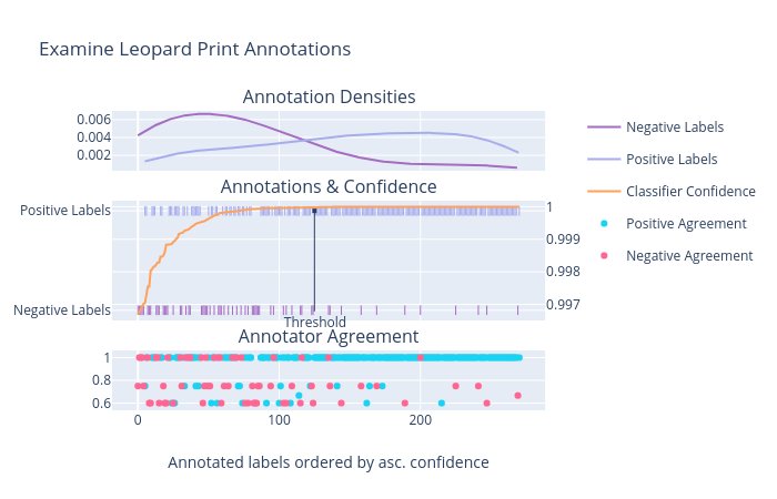
Below we present an annotation plot for a run of our EM algorithm for a leopard print image classifier, which is a binary classifier and has a single class output. The middle subplot presents the annotations for the images sent to a crowdsourcing platform, ordered in ascending class-confidence score (as illustrated by the orange curve), where positive labeled images are indicated at the top of the subplot by blue dashes and negative labelled images are indicated at the bottom of the subplot by purple dashes. We can see that for high confidence predictions there are many positive annotations with few negative annotations, illustrating that the classifier is performing well. However there is a point at which the occurrence of positive labels is frequently punctuated by negative annotations, illustrating that the classifier performs poorly beyond this point. We can see from the subplot that the threshold estimated by the EM algorithm (as indicated by the black dot) is positioned just before the classifier begins to perform poorly, which demonstrates the algorithm's usefulness in estimating an optimal class-confidence threshold. Furthermore, the annotation density subplot indicates a natural separation between the cluster of positive and negative annotations, and the estimated threshold corresponds to this also.
To illustrate further we present a slope plot below, where we generate a cumulative sum of annotations and examine the slope of the curve, where annotations are assigned values 1 & 0 for positive and negative labels respectively, and are ordered by the class-confidence scores generated by the classifier (as was the case in the previous plot). The resultant plot is piecewise linear, where flat-line segments in the curve above the threshold represent consecutive False Positives, whereas those beneath the threshold represent consecutive True Negatives. Conversely, sloped-line segments in the curve above the threshold represent consecutive True Positives, whereas those beneath the threshold represent consecutive False Negatives. For our purposes we would like the curve above the threshold to have a slope as close to 1 as possible, and on average to have a steeper slope above the threshold than beneath it.

In the slope plot we observe the following:
- There are many long sloped-line segments above the threshold, whereas there are few beneath the threshold
- There are many long flat-line segments beneath the threshold, whereas there are few above the threshold
- The slope on average above the threshold is steeper than beneath it
Therefore, for the leopard print image classifier predictions, we see that the threshold estimated by the AutoThreshold algorithm successfully identifies an appropriate class-confidence threshold.
Conclusion
We have presented a novel algorithm for the task of optimal threshold estimation for an image classifier that is applied to out-of-distribution data, where an EM algorithm and human-in-the-loop is used to generate annotations for the out-of-distribution data, which are used to calculate a threshold to compensate for the difference in distributions. The algorithm is simple to implement, and is efficient in terms of the number of annotated image examples required to estimate an optimal threshold.
In future work, we will explore using the EM algorithm and human-in-the-loop to train a classifier in the context of active learning, i.e., the case where there is no annotated data set to train a classifier.
If you would like to work on similar problems, consider joining our Data Science teams!
Appendix A: Mathematical Details
Below we provide further details on the presented algorithm's interpretation as an Expectation-Maximization (EM) algorithm.
EM Algorithm Description
Using standard notation, the EM algorithm can be described as follows: For a set of observed data \(\mathbf{X}\) generated from a statistical model with unknown parameters \(\boldsymbol{\theta}\), and a set of latent variables \(\mathbf{Z}\), which are unobserved but effect the distribution of the data nonetheless, we estimate the values for \(\boldsymbol{\theta}\) by maximizing the marginal likelihood of the observed data,
\({\displaystyle L({\boldsymbol {\theta }};\mathbf {X} )=p(\mathbf {X} \mid {\boldsymbol {\theta }})=\int p(\mathbf {Z} \mid \mathbf {X} ,{\boldsymbol {\theta }})p(\mathbf {X} \mid {\boldsymbol {\theta }})\,d\mathbf {Z} }\),
i.e, we generate a maximum likelihood estimate (MLE) for \(\boldsymbol{\theta}\). However, this quantity is often intractable since \(\mathbf {Z}\) is unobserved and its distribution is unknown before obtaining \(\boldsymbol{\theta}\).
The EM algorithm seeks to overcome this issue, and finds the MLE of the marginal likelihood by iteratively maximizing a specifed \(Q\) function, which is defined as the expected value of the log likelihood function of \({\boldsymbol {\theta }}\), i.e., \(Q({\boldsymbol {\theta }}\mid {\boldsymbol {\theta }}^{(t)})=\operatorname {E} _{\mathbf {Z} \mid \mathbf {X} ,{\boldsymbol {\theta }}^{(t)}}\left[\log L({\boldsymbol {\theta }};\mathbf {X} ,\mathbf {Z} )\right]\,\). The \(Q\) function is maximized over two steps: In the first step—the E-step—the data-dependent parameters of the \(Q\) function are calculated, while in the second step—the M-step—we seek to maximize the function constructed in the E-step over the parameters \(\boldsymbol{\theta}\), where the value that achieves the maximum is our new estimate, \(\boldsymbol {\theta }^{(t)}\).
AutoThreshold as an EM Algorithm
Using the above notation and translating to our algorithm description, our observations, \(\mathbf{X}\), are the vector of annotations generated by human-in-the-loop, \(\mathbf{a}\); our unobserved latent variables, \(\mathbf{Z}\), are the ordered classifier predictions used to generate \(\mathbf{a}\), i.e. \(\mathbf{p}\); and the unknown model parameters, \({\boldsymbol {\theta }}\), are defined by the statistical model used to generate \(\mathbf{X}\), which in our case is the Bernoulli distribution, as the annotators answer a yes-no question when generating annotations for our image data set. For the Bernoulli distribution, there is single model parameter \(p\), which is simply the probability that an observation will be true.
For our use case, where we estimate a class-confidence threshold, \(\hat{t}\), for an image classifier in order to generate binary predictions, the parameter \(p\) has a direct correspondence, which can be explained as follows: For an ideal image classifier with perfect accuracy applied to a balanced data set (i.e., a data set with an equal number of true and false examples) the output distribution of the class labels will be uniform and the parameter \(p\) will be 0.5, as all predictions will be correct, and a true or false outcome will have equal probability as the observations are balanced. Similarly, in the ideal case the sigmoid units at the output will be perfectly normalized and the class-confidence threshold used to assign predictions to categories will also be 0.5 (as is the standard assumption with logistic regression analysis etc.). Also, 0.5 corresponds to the sample mean of the observed predictions (where true & false are represented numerically by 1 & 0) which is the MLE for the parameter \(p\).
Known Unknowns
As we move away from the ideal case where the data may not be balanced or the image classifier may exhibit errors, the parameter \(p\) and threshold \(t\) deviate from 0.5 and both become unknown (but still remain in the range from 0 to 1), since the classifier's output class distribution, \(\mathbf{y}\), becomes unknown. However, a direct correspondence between the two parameters remains. To overcome this issue, and estimate an appropriate value for \(t\) using a known distribution, i.e., \(\hat{t}\), we generate a validation data set, i.e., a set of manually annotated images, and test the image classifier by generating class predictions for the images then compare against the image annotations. The goal is to estimate a value for \(\hat{t}\) that will generate a class label output distribution, \(\mathbf{y}\), as close as possible to \(\mathbf{a}\).
However, as already discussed in this article, there are additional practical considerations when evaluating the performance of an image classifier such as precision & recall, and simply comparing annotations to class predictions to determine performance may not lead to the selection of a useful classifier. To choose a suitable image classifier, the effect of the class-confidence threshold itself must be considered, which leads to a meta-labeling of the model's class predictions using the annotations in the validation data set. In particular, all positively annotated images that are correctly classified are known as True Positives (TP), whereas those that are incorrectly classified are known as False Negatives (FN). Conversely, all negatively annotated images that are correctly classified are known as True Negatives (TN), whereas those that are incorrectly classified are known as False Positives (FP).
Using these four categories of class prediction, a performance metric can indicate how close an image classifier's class output distribution is to the validation data set, while also giving an indication of the classifier's performance when it comes to precision & recall.
Averages Over Categories
As mentioned above an important component of the EM algorithm is how to calculate the maximum likelihood estimate for the unknown parameter \(\boldsymbol{\theta}\). For our use case where the observations are generated by a Bernoulli distribution, the MLE for the parameter \(p\) is the sample mean. Although, as discussed above, for our use case we must also consider precision & recall, which necessitates the use of a performance metric to determine a class-confidence threshold that optimizes \(p\) with respect to the validation data set. However, performance metrics such as precision & recall can be interpreted as averages over categories, which provides a direct connection to the MLE for \(p\). For example, recall can be considered an average over the meta-labeled positive annotations TP & FN, i.e., recall = TP/(TP+FN); while precision can be considered an average over the meta-labeled annotations above the threshold, i.e., precision = TP/(TP+FP). Furthermore, as discussed, precision and recall may be combined to create a performance metric such as the \(f_\beta\)-measure, such derived performance metrics also perform averaging over the values for precision & recall. In summary, for a chosen performance metric, the optimal value for \(\hat{t}\) has the effect of generating a Bernoulli distribution \(\mathbf{y}\) which is a close as possible to \(\mathbf{a}\), and also specifies a level of control over precision and recall.
Optimization Loop
Now that we have described how the AutoThreshold algorithm fits within the framework of the EM algorithm, we will provide further detail on the algorithm's optimization loop.
At each iteration, the number of items in \(\mathbf{a}\), and their corresponding \(\mathbf{p}\), increases by our specified window size, \(m\), which increases the amount of data available to calculate our specified performance metric, \({\tt metric}(.)\), and also increases the number of possible values to be used to maximize \(\hat{t}\). Where we increase the available observations in the E-step (by generating new annotations from our most confident predictions) and maximize the threshold in the M-step to estimate the optimal threshold. Here the E-step is arguably most important, since it generates the required validation data set, as the original problem is to generate a sufficient number of annotations for an unannotated data set to estimate a threshold. Furthermore, in the E-step, we increase the available observations using a suitably large subset size until the algorithm converges, which allows us to minimize overall the number of annotations needed to estimate an optimal threshold, which is what we wish to achieve with this algorithm.
Finally
To conclude we present some other interesting points to consider about this algorithm:
For this use case we apply the EM algorithm to a discrete probability distribution using categorical observations, i.e., annotations. Typically EM is applied to problems where observations are drawn from a continuous probability distribution, such as the Gaussian distribution.
For this use case we have our latent variables, \(\mathbf{p}\), before we obtain our observations, \(\mathbf{a}\). This is the reverse of the standard implementation of EM, and illustrates the flexibility of the EM algorithm's two-step learning iteration when applied to human-in-the-loop.
For this use case we have human-generated observations, where usually the EM algorithm is applied to sensor observations.
Appendix B: AutoThreshold Python Implementation
Below we present a simple code implementation of the AutoThreshold algorithm applied to a binary classification task using synthetic data.
#!/usr/bin/env python3.8

import numpy as np
from collections import namedtuple
from sklearn.metrics import f1_score

SyntheticData = namedtuple('SyntheticData', ['predictions', 'annotations'])

def generate_predictions_and_annotations(n):
    """Returns synthetic predictions and annotations for a step classifier response,
    ordered by prediction score.

    Note: The returned synthetic data has an optimal threshold at 0.5

    """
    predictions = np.linspace(0, 1, n)
    annotations = np.concatenate((np.zeros(n//2), np.ones(n//2)))
    return SyntheticData(predictions, annotations)

def predictions_generator(synthetic_data, thresh_ind):
    """Returns predictions for the current subset window as specified by `thresh_ind`.

    Note: In the normal operation of AutoThreshold this step would generate predictions
    for our out-of-distribution images from our image classifier. Here, our toy example
    is run on synthetic data and our precomputed predictions are simply returned.
    """
    return synthetic_data.predictions[thresh_ind-M//2:thresh_ind+M//2]

def annotations_generator(synthetic_data, thresh_ind):
    """Returns annotations for the current subset window as specified by `thresh_ind`.

    Note: In the normal operation of AutoThreshold this step would source annotations
    from a crowdsourcing platform. Here, our toy example is run on synthetic data and
    our precomputed annotations are simply returned.
    """
    return synthetic_data.annotations[thresh_ind-M//2:thresh_ind+M//2]

def calculate_optimal_threshold(annotations, predictions):
    """Returns the index of the optimal threshold using the F1 score.

    **Example:**

    >>> predictions = [0, 0.2, 0.4, 0.6, 0.8, 1.0]
    >>> annotations = [0, 0, 0, 1, 1, 1]
    >>> thresh_ind = calculate_optimal_threshold(annotations, predictions)
    >>> threshold = predictions[thresh_ind]
    >>> threshold
    0.6
    """
    scores = []
    for threshold in predictions:
        labels = []
        for prediction in predictions:
            label = 1 if prediction >= threshold else 0
            labels.append(label)
        scores.append(f1_score(annotations, labels))
    return np.argmax(scores)

def auto_threshold(synthetic_data, annotation_generator):
    """Main loop of the AutoThreshold algorithm.
    """
    # Specify initial estimate; here we start from the highest confidence which is
    # the n-th ordered prediction
    thresh_ind = N
    thresh_est = synthetic_data.predictions[thresh_ind-1]

    for i in range(MAX_ITERS):

        # E-Step: Generate annotations for the subset of ordered predictions
        predictions_subset = predictions_generator(synthetic_data, thresh_ind)
        annotations_subset = annotations_generator(synthetic_data, thresh_ind)

        # M-Step: Estimate local threshold index for the newly annotated subset
        thresh_ind_subset = calculate_optimal_threshold(annotations_subset, predictions_subset)

        # Estimate new threshold
        thresh_ind_old = thresh_ind
        thresh_ind = (thresh_ind_old - M//2) + thresh_ind_subset
        thresh_est = synthetic_data.predictions[thresh_ind]

        print('Iter: {}, Est: {:.3f}'.format(i, thresh_est))

        # Check convergence
        if thresh_ind == thresh_ind_old:
            print('Converged')
            break

    return thresh_est

if __name__ == "__main__":

    print("\nAutoThreshold Toy Example.\n")

    # Specify arguments: Max algorithm iterations, number of synthetic predictions & subset size
    MAX_ITERS = 25; N = 10000; M = 500

    # Synthetically generate ordered classifier predictions and annotations
    synthetic_data = generate_predictions_and_annotations(N)

    # Run AutoThreshold to estimate optimal classifier threshold
    thresh_est = auto_threshold(synthetic_data, annotations_generator)
    print("\nEstimated threshold value: {:.3f}".format(thresh_est))

    print("\n\tFin.\n")
Code output will look like:
$ ./autothreshold.py
AutoThreshold Toy Example.

Iter: 0, Est: 0.975
Iter: 1, Est: 0.950
Iter: 2, Est: 0.925
Iter: 3, Est: 0.900
Iter: 4, Est: 0.875
Iter: 5, Est: 0.850
Iter: 6, Est: 0.825
Iter: 7, Est: 0.800
Iter: 8, Est: 0.775
Iter: 9, Est: 0.750
Iter: 10, Est: 0.725
Iter: 11, Est: 0.700
Iter: 12, Est: 0.675
Iter: 13, Est: 0.650
Iter: 14, Est: 0.625
Iter: 15, Est: 0.600
Iter: 16, Est: 0.575
Iter: 17, Est: 0.550
Iter: 18, Est: 0.525
Iter: 19, Est: 0.500
Iter: 20, Est: 0.500
Converged

Estimated threshold value: 0.500

        Fin.
We're hiring! Do you like working in an ever evolving organization such as Zalando? Consider joining our teams as a Machine Learning Engineer!


